| Oracle® Retail Demand Forecasting User Guide for the RPAS Fusion Client Release 16.0 E91109-03 |
|

 Previous |
 Next |
| Oracle® Retail Demand Forecasting User Guide for the RPAS Fusion Client Release 16.0 E91109-03 |
|
Previous |
Next |
The Forecast Administration task allows you to set up RDF to generate forecasts.
This section describes the components of the Forecast Administration.
Forecast Administration is the first task used in setting up RDF to generate forecasts. It provides access to forecast settings and parameters that govern the whole domain (database). These settings and parameters are divided into two areas, Basic and Advanced, and are available beneath the Forecast Administration task.
The Basic Settings are used to establish a final-level forecast horizon, the commencement and frequency of forecast generation, and the specification of aggregation levels (Source Levels) and spreading (Profile) methods used to yield the final-level forecast results. For information on the views in Basic Settings, refer to Forecast Administration Workbook: Basic Settings.
The Advanced Settings are used to set default values for parameters affecting the algorithm and other forecasting techniques used to yield final-level and source-level forecasts, thus eliminating the need to define these parameters individually for each product and location. If certain products or locations require parameter values other than the defaults, these fields can be amended on a case-by-case basis in the Forecast Maintenance Workbook. For information on the views in Advanced Settings, refer to Forecast Administration Workbook: Advanced Settings.
Often, forecast information is required for items at a very low level in the hierarchy. However, problems can arise in that data is often too sparse and noisy to identify clear patterns at these lower levels. For this reason, it sometimes becomes necessary to aggregate sales data from a low level to a higher level in the hierarchy in order to generate a reasonable forecast. Once this forecast is created at the higher or source-level, the results can be allocated to the lower-level or final-level dimension based on the lower level's relationship to the total.
In order to spread this forecast information back down to the lower level, it is necessary to have some idea about the relationship between the final-level and the source-level dimensions. Often, an additional interim forecast is run at the low level in order to determine this relationship. Forecast data at this low level might be sufficient to generate reliable percentage-to-whole information, but the actual forecast numbers are more robust when generated at the aggregate level.
The Final Level view represents forecast parameters for the lower (final) level, the level to which source forecast values are ultimately spread. Forecast data must appear at some final-level in order for the data to be approved or exported to other systems. The Source Level view represents the default values for forecast parameters at the more robust aggregate (source) level.
A forecasting system's main goal is to produce accurate predictions of future demand. The RDF solution utilizes the most advanced forecasting algorithms to address many different data requirements across all retail verticals. Furthermore, the system can be configured to automatically select the best algorithm and forecasting level to yield the most accurate results.
Following is a summary of the various forecasting methods employed in RDF. Some of these methods may not be visible in your solution based on configuration options set in the RPAS Configuration Tools. More detailed information on these forecasting algorithms is provided inChapter 3, "Oracle Retail Demand Forecasting Methods"
Average
RDF uses a simple average model to generate forecasts.
Moving Average
RDF uses a simple moving average model to generate forecasts. You can specify a Moving Average Window length.
IntermittentES
RDF fits the data to the Croston's model of exponential smoothing. This method should be used when the input series contains a large number of transitions from non-zero sales to zero data points (that is, intermittent demand data). The original time series is split into a Magnitude and Frequency series, and then the SimpleES model is applied to determine level of both series. The ratio of the magnitude estimate over the frequency estimate is the forecast level reported for the original series.
TrendES
RDF fits the data to the Holt model of exponential smoothing. The Holt model is useful when data exhibits a definite trend. This method separates base demand from trend and then provides forecast point estimates by combining an estimated trend and the smoothed level at the end of the series. For instance, where the forecast engine cannot produce a forecast using the TrendES method, the Simple/IntermittentES method is used to evaluate the time series.
Causal
Causal is used for promotional forecasting and can only be selected if Promote is implemented. Causal uses a Stepwise Regression sub-routine to determine the promotional variables that are relevant to the time series and their lift effect on the series. AutoES and source-level forecasting are used to generate future baseline forecasts. By combining the future baseline forecast and each promotion's effect on sales (lift), a final promotional forecast is computed. For instances where the forecasting engine cannot produce a forecast using the Causal method, the system evaluates the time series using the SeasonalES method.
To forecast short lifecycle, promotional items, Causal deprices, depromotes, and smoothes the forecasting data source to generate the short-lifecycle forecast causal baseline. The promotion effects are calculated using the same Stepwise Regression code as Causal. However, the promo lifts are first filtered from the sales and applied on top of the item's rate of sale. The resulting measure is regressed against the promotional variables to determine the promotion effects. Finally, the promotion effects are applied on top of the short lifecycle baseline to generate the final forecast.
No Forecast
No forecast is generated for the product/location combination.
Bayesian
Useful for short lifecycle forecasting and for new products with little or no historic sales data, the Bayesian method requires a product's known sales plan (created externally to RDF) and considers a plan's shape (the selling profile or lifecycle) and scale (magnitude of sales based on Actuals). The initial forecast is equal to the sales plan, but as sales information comes in, the model generates a forecast by merging the sales plan with the sales data. The forecast is adjusted so that the sales magnitude is a weighted average between the original plan's scale and the scale reflected by known history. A Data Plan must be specified when using the Bayesian method. For instances where the Data Plan equals zero (0), the system evaluates the time series using the SeasonalES method.
Profile-based
RDF generates a forecast based on a seasonal profile that can be created in RPAS or legacy system. Profiles can also be copied from another profile and adjusted. Using historic data and the profile, the data is de-seasonalized and then fed to the SimpleES method. The Simple forecast is then re-seasonalized using the profiles. A Seasonal Profile must be specified when using the Profile-Based method. For instances where the Seasonal Profile equals zero, the system evaluates the time series using the SeasonalES method.
Components
The Components forecast method multiplies pre-calculated baseline, promotional lifts, and regular price lifts to generate the forecast. These components are specified in Forecast Administration task, Advanced Settings activity, Final Level Parameters view. The following table lists the components and their referenced measures.
| Component | Measure |
|---|---|
| Baseline | Components - Baseline |
| Regular Price Lifts | Components - Regular Price Lifts |
| Promotional Lifts | Components - Promotional Lifts |
| Interval | Components - Baseline Interval |
Intervals are not generated and need to be provided. This method is useful when the forecast components are available since the forecast can be quickly generated.
Automatic Exponential Smoothing (AutoES)
RDF fits the sales data to a variety of exponential smoothing models of forecasting, and the best model is chosen for the final forecast. The candidate methods considered by AutoES are:
The final selection between the models is made according to a performance criterion (Bayesian Information Criterion) that involves a trade-off between the model's fit over the historic data and its complexity.
SimpleES
RDF uses a simple exponential smoothing model to generate forecasts. SimpleES ignores seasonality and trend features in the demand data and is the simplest model of the exponential smoothing family. This method can be used when less than one year of historic demand data is available.For more information, see Simple Exponential Smoothing.
Croston's Method
Croston's Method is used when the input series contains a large number of transitions from non-zero sales to zero data points (that is, intermittent demand data). For more information, see Croston's Method.
Simple/IntermittentES
Simple/IntermittentES is a combination of the SimpleES and IntermittentES methods. This method applies the SimpleES model unless a large number of transitions from non-zero sales to zero data points are present, in which case the Croston's model is applied.For more information, see Simple/Intermittent Exponential Smoothing.
HoltES
Holt exponential smoothing treats data as linearly trended but non-seasonal. The Holt model provides forecast point estimates by combining an estimated trend (for the forecast horizon - h) and the smoothed level at the end of the series. RDF uses a damped Holt model that decays the trend component so that it disappears over the first few weeks. This improves forecasts created using Holt over longer forecast horizons.For more information, see Holt Exponential Smoothing.
Multiplicative Seasonal
Also referred to as Multiplicative Winters Model, this model extracts seasonal indices that are assumed to have multiplicative effects on the un-seasonalized series.For more information, see Multiplicative Winters Exponential Smoothing which includes:
Oracle Winters
Oracle Winters Decomposition
Winters Standard
Winters Responsive
Additive Seasonal
Also referred to as Additive Winters Model, this model is similar to the Multiplicative Winters model, but is used when zeros are present in the data. This model adjusts the un-seasonalized values by adding the seasonal index (for the forecast horizon). For more information, see Additive Winters Exponential Smoothing.
SeasonalES
This method, a combination of several Seasonal methods, is generally used for known seasonal items or forecasting for long horizons. This method applies the Multiplicative Seasonal model unless too many zeros are present in the data, in which case the Additive Winters model of exponential smoothing is used. If less than two years of data is available, a Seasonal Regression model is used. If there is too little data to create a seasonal forecast (in general, less than 52 weeks), the system selects from the SimpleES, TrendES, and IntermittentES methods. For more information, see Seasonal Exponential Smoothing (SeasonalES).
Seasonal Regression
Seasonal Regression cannot be selected as a forecasting method, but is a candidate model that is used only when the SeasonalES method is selected. This model requires a minimum of 52 weeks of history to determine seasonality. Simple Linear Regression is used to estimate the future values of the series based on a past series.
The independent variable is the series history one-year or one cycle length prior to the desired forecast period, and the dependent variable is the forecast. This model assumes that the future is a linear combination of itself one period before plus a scalar constant. For more information, see Seasonal Regression.
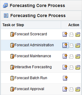
To build the Forecast Administration workbook, perform these steps:
Click the New Workbook icon in the Forecast Administration task in the Forecasting Core Process activity.
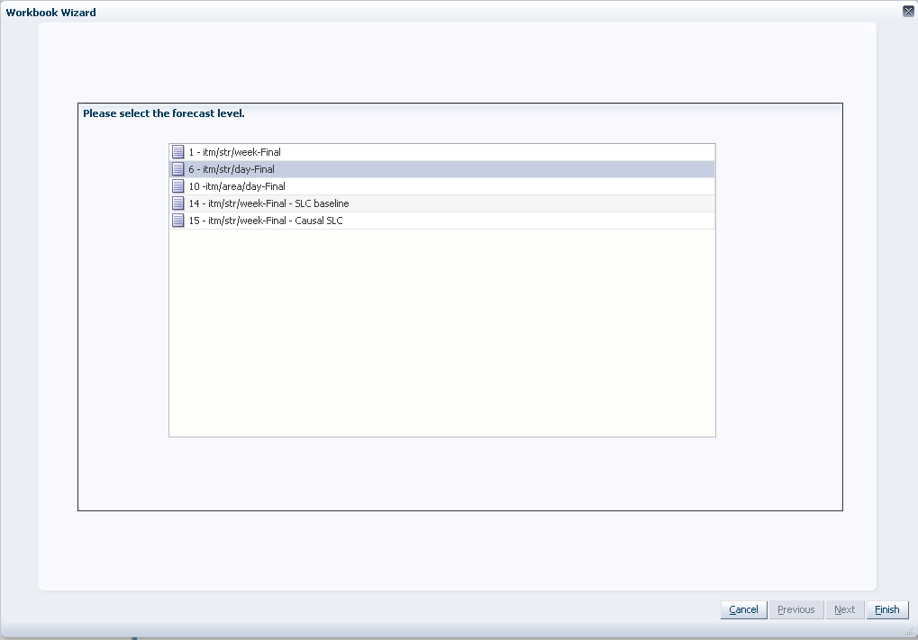
The Workbook wizard opens. Select the forecast level you want to work with and click Finish.
|
Note: The final forecast level is a level at which approvals and data exports can be performed. Depending on your organization's setup, you may be offered a choice of several final forecast levels. Make the appropriate selection. |
The Forecast Administration workbook is built.
The Forecast Administration Basic Settings workbooks contains two views:
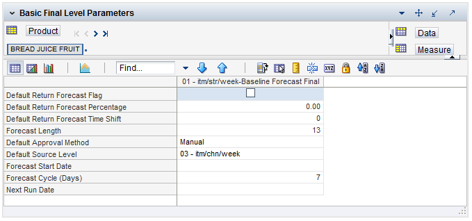
The Final Level view allows you to set the forecast horizon information, frequency of review, and all default parameters for the lower or final-level forecast (the level to which aggregate forecast data is ultimately spread). Forecast approvals and data exports can only be performed on forecasts at a final-level. Figure 8-3 provides an example of a view of the Final Level Parameters view in a master domain with three partitions/local domains, partitioned based on group.
The Final Level View - Basic Settings contains the following measures:
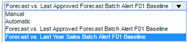
Default Approval Method
This field is a list from which you select the default automatic approval policy for forecast items. Valid values are:
| Field | Description |
|---|---|
| Manual | The system-generated forecast is not automatically approved. Forecast values must be manually approved by accessing and amending the Forecast Approval Workbook. |
| Automatic | The system-generated quantity is automatically approved as is. |
| By Alert | This list of values may also include any Forecast Approval alerts that have been configured for use in the forecast approval process. Alerts are configured during the implementation and can be enabled to be used for Forecast Approval in the Enable Alert for Forecast Approval view. Refer to the Oracle Retail Predictive Application Server Configuration Tools User Guide for more information on the Alert Manager. The Alert Parameters workbook contains a list and descriptions of available alerts, and for which level (causal/baseline) that they are designed for. |
Default Return Forecast Flag
If this Boolean measure is checked, it indicates that a returns forecast will be generated.
Default Return Forecast Percentage
This measure indicates the percentage of the merchandise sold in a time period that is expected to be returned to the store. A value of zero indicates that no returns will be calculated.
Default Return Forecast Time Shift
This measure indicates the number of time periods between when the merchandise was sold until it was returned. For instance, if the measure is set to one, the merchandise is expected to be returned one week after it was sold.
Default Source Level
The pick list of values displayed in this field allows you to change the forecast level that is used as the primary level to generate the source forecast. The source-levels are set up in the RPAS Configuration Tools. A value from the pick list is required in this field at the time of forecast generation.
Forecast Cycle
The Forecast Cycle is the amount of time (measured in days) that the system waits between each forecast generation. Once a scheduled forecast has been generated, this field is used to automatically update the Next Run Date field. A non-zero value is required in this field at the time of forecast generation.
Forecast Start Date
This is the starting date of the forecast. If no value is specified at the time of forecast generation, the system uses the data/time at which the batch is executed as the default value. If a value is specified in this field and it is used to successfully generate the batch forecast, this value is cleared.
Forecast Length
The Forecast Length is used with the Forecast Start Date to determine forecast horizon. The forecast length is based on the calendar dimension of the final-level. For example, if the forecast length is to be 10 weeks, the setting for a final-level at day is 70 (10 x 7 days).
Next Run Date
The Next Run Date is the date on which the next batch forecast generation process automatically runs. RDF automatically triggers a set of batch processes to be run at a pre-determined time period. When a scheduled batch is run successfully, the Next Run Date automatically updates based on the Start Date value and the Forecast Cycle. No value is required in this field when the Forecast Batch Run Workbook wizard is used to generate the forecast or if the batch forecast is run from the back-end of the domains using the override True option. Refer to the Oracle Retail Demand Forecasting Implementation Guide for more information on forecast generation.
Enable New Item Functionality
The New Item functionality is not automatically available for every forecast level. You can enable it for a certain level by checking this measure.
Causal Run Mode
|
Note: This measure is not displayed for baseline levels. |
Allows you to select the default behavior of the causal engine. The are three options:
Run Pooling Estimation — the promotion effects are estimated at the specified source levels. No forecast is generated.
Run Forecast — the promotion effects are estimated at the final forecast level. Then, if specified, the promotion effects from the final and source levels are blended. Finally, the blended promotion effects are used to generate the forecast.
Run Both — the causal engine will performs all the actions described in the other options.
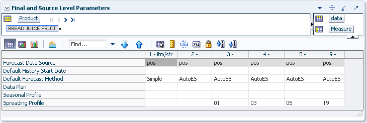
The Final and Source Level view allows you to set the default parameters that are common to both the final and source-level forecasts.
The Final and Source Level Parameters View - Basic Settings contains the following measures:
Forecast Data Source
This is a read-only value that displays the sales measure (the measure name) that is the data used for the generation of forecasts (for example, POS). The measure that is displayed here is determined at configuration time in the RPAS Configuration Tools. Different Data Sources can be specified for the Final and Source Levels.
Default History Start Date
This field indicates to the system the point in the historical sales data at which to use in the forecast generation process. If no date is indicated, the system defaults to the first date in your calendar. It is also important to note that the system ignores leading zeros that begin at the history start date. For example, if your history start date is January 1, 2011 and an item/location does not have sales history until February 1, 2011, the system considers the starting point in that item/location's history to be the first data point where there is a non-zero sales value. Different History Start Dates can be specified for the Final and Source Levels.
Data Plan
|
Note: This measure is not displayed for causal levels. |
Used in conjunction with the Bayesian forecast method, Data Plan is used to input the measure name of a sales plan that should be associated with the final-level forecast. Sales plans, when available, provide details of the anticipated shape and scale of an item's selling pattern. If the Data Plan is required, this field should include the measure name associated with the Data Plan.
Default Forecast Method
|
Note: If this a Causal forecast level, then the only available methods are Causal and No Forecast. Alternately, when the level is non-causal, the Causal method is not available. |
The Default Forecast Method is a complete list of available forecast methods from which you can select the primary forecast method that is used to generate the forecast. A summary of methods is provided in Forecasting Methods Available in RDF. The chapter, "Oracle Retail Demand Forecasting Methods", covers each method in greater detail.
It is important to note that Causal should not be selected unless the forecast level was set as a Causal level during the configuration. Refer to the Oracle Retail Demand Forecasting Configuration Guide for more information on configurations using the Causal forecast method.
Seasonal Profile
|
Note: This measure is not displayed for causal levels. |
Used in conjunction with the Profile-Based forecasting method, this is the measure name of the seasonal profile that is used to generate the forecast at either the source or final-level. Seasonal profiles, when available, provide details of the anticipated seasonality (shape) of an item's selling pattern. The seasonal profile can be generated or loaded, depending on your configuration. The original value of this measure is set during the configuration of the RDF solution.
Spreading Profile
|
Note: This measure is not displayed for causal levels. |
Used for source-level forecasting, the value of this measure indicates the profile level that is used to determine how the source-level forecast is spread down to the final-level. No value is needed to be entered at the final-level. For dynamically generated profiles, this value is the number associated with the final profile level (for example, 01). Note that profiles one (1) through 9 have a zero (0) preceding them in Curve—this is different than the forecasting level numbers.
For profiles that must be approved, this is the measure associated with the final profile level. This measure is defined as apvp +level (for example, apvp01 for the approved profile for level 01 in Curve).
Source Level Forecast Data Source
You can specify a measure to serve as a forecast data source at the source-level. If the measure is left blank for a certain source-level, the source measure from the corresponding final-level is used.
Source Level History Start Date
This is the starting date for historical sales data at the source-level. For example, if your system start date is January 1, 2003, but you only want to use historical sales data from the beginning of 2011, you need to set your History Start Date to January 1, 2011. Only history after this date is used for generating the forecast. The default is the system start date unless otherwise specified. If sales data is collected weekly or monthly, RDF generates forecasts only using data from sales periods after the one containing the history start date.
It is also important to note that the system ignores leading zeros that begin at the history start date. For example, if your history start date is January 1, 2011, and an item/location does not have sales history until February 1, 2011, the system considers the starting point in that item/location's history to be the first data point where there is a non-zero sales value.
|
Note: History start dates for final and source-levels can be different. |
The Forecast Administration Advanced Settings workbooks contain these views:
The Forecast Administration Advanced Settings workflow activity is used to set parameters related to either the data that is stored in the system or the forecasting methods that are used at the final or source-levels. The parameters on this workflow activity are not as likely to be changed on a regular basis as the ones on the Basic Settings workflow activity.
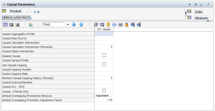
The Causal Parameters view allows you to set the parameters that support promotional forecasting. The parameters that support overlapping promotions are also specified in this view. Overlapping promotions are promotions that happen at the same time period at the same location for the same product. This view only includes the causal forecast levels for the final-level selected during the wizard process. This view is not visible if Promote/Promotional Forecasting is not implemented in your RDF environment.
The Causal Parameters View - Advanced Settings contains the following measures:
Aggregated Promotional Lift Override
This parameter contains the name of the measure that stores the higher level (aggregated) promotional peak override. The name is implementation specific. If populated, during the causal forecasting generation the aggregated lift is spread down to the appropriate final level intersection.
Causal Aggregation Profile
Used only for Daily Causal Forecasting, the Causal Aggregation Profile is measure name of the profile used to aggregate promotions defined at day up to the week. The value entered in this field is the measure name of profile. If this profile is generated within Curve, the format of the measure name is apvp+level (for example, apvp01). Note that the only aggregation of promotion variables being performed here is along the Calendar hierarchy. RDF does not support aggregation of promotion variables along other hierarchies such as product and location hierarchies.
Causal Beta Scale
As part of the causal forecasting process, the average sales of non-promo periods in history are divided by the Beta Scale. If the resulting ratio is less than beta zero, the causal forecasting method succeeds. If not, the causal forecasting method fails and the baseline serves as the forecast for the time series.
Causal Calculation Intersection
Used only for Daily Causal Forecasting, the Causal Calculation Intersection is the intersection at which the causal forecast is run. The format needs to match the hierarchy dimension names set in the RPAS Configuration Tools (such as itemstr_week). Each dimension must have only four characters. The order of the dimension does not matter. There is no validation of correct format of this intersection.
|
Note: When using Daily Causal Forecasting, it is recommended that the calculation is performed at the week level. |
Causal Calculation Intersection Periodicity
This measure is obsolete if a baseline forecast is provided to the causal calculation. Used only for Daily Causal Forecasting, the Causal Calculation Intersection Periodicity must be set to the periodicity of Causal Calculation Intersection. Periodicity is the number of periods within one year that correspond to the calendar dimension (for example, 52 if the Causal Calculation Intersection is defined with the week dimension).
Causal Capping Number
The value of this parameter is a measure based on the same product and location intersection as the forecast level. The maximum value of the referenced measure times the Causal Capping Ratio is the maximum value to use for calculating the causal forecast for time series that meet the Causal Capping conditions. If Use Causal Capping is set to True, the history for the time series is greater than or equal to the Minimum Causal Capping History, and the preliminary forecast is greater than or equal to the value in the Causal Capping Number measure times the Causal Capping Ratio, then the forecast is recalculated to be the value in the Causal Capping Number measure multiplied by the value in the Causal Capping Ratio measure.
Causal Capping Ratio
The value of this parameter is a measure based on the same product and location intersection as the forecast level. This measure contains the ratio that is used to calculate the forecasts for time series that meet the Causal Capping conditions. If Use Causal Capping is set to True, the history for the time series is greater than or equal to the value in the Minimum Causal Capping History measure, and the preliminary forecast is greater than or equal to the value in the Causal Capping Number measure times the Causal Capping Ratio, then the forecast is recalculated to be the Causal Capping Number multiplied by the value in the Causal Capping Ratio measure.
Causal Data Source
Used only for Daily Causal Forecasting, the Causal Data Source is an optional setting that contains the measure name of the sales data to be used if the data for causal forecasting is different than the Data Source specified at the Final level. If needed, this field should contain the measure name of the source data measure (for example, DPOS).
If set to True, Seasonal Regression is excluded from the choice of methods for baseline calculation within Causal.
|
Note: This parameter does not impact the choice of forecast methods within SeasonalES. |
Causal Baseline
Enter the measure name that you want to serve as the baseline for the causal forecast at this level.The measure can be loaded or it can be generated in a different forecast run.
Causal Higher Intersection
An optional setting for Causal Forecasting, this intersection is the aggregate level to model promotions if the causal intersection cannot produce a meaningful causal effect. This intersection applies to promotions that have a Promotion Type is set to Override From Higher Level (set in the Promo Effect Maintenance Workbook). The format of this intersection needs to match the hierarchy dimension names set in the RPAS Configuration Tools such as sclsrgn_ (Subclass/Region), and it must not contain the calendar dimension. Each dimension must have only four characters. The order of the dimension does not matter. There is no validation of correct format of this intersection.
Causal Spread Profile
Used only for Daily Causal Forecasting, the Causal Spread Profile is the measure name of the profile used to spread the causal baseline forecast from the Causal Calculation Intersection to the Final Level. If this profile is generated in Curve, this measure value is apvp+level (for example, apvp01).
Default Overlapping Promotion Adjustment Factor
The Overlapping Promotion Behavior measure is applied only if Adjustable Approach is selected for Default Overlapping Promotions Behavior.
This Default Overlapping Promotion Adjustment Factor specifies at a high level how the individually calculated promotions interact with each other when they are overlapping in the forecast horizon. This parameter serves as a global setting, but can be overridden at lower levels. The default value is 1.
A value greater than 1 means the promotion effects will be compressed when applied in the model, instead of linearly summing up to get the total promotion effect. The larger the value is, the larger the compression effect will be, meaning the smaller the total effect will be.
A value between 0 and 1 means the promotion effects will be amplified when applied in the model, instead of linearly summing up to get the total promotion effect. The smaller the value is, the larger the amplification effect will be, meaning the larger the total effect will be.
If a value less than or equal to 0 is put in the cell, the calculation engine will find the best adjustment factor to fit the history data. This factor is then used to combine overlapping promotions in the forecast horizon. With few exceptions, the value should be anywhere from 1 to 5. This factor is then used to combine overlapping promotions in the forecast horizon
|
Caution: The process to find the best adjustment factor can be time consuming and introduce performance issues. |
Default Overlapping Promotions Behavior
The Overlapping Promotion Behavior measure allows you to specify if overlapping promotions function should be activated during the batch run. If so, the causal algorithm will create a new promotion for each unique combination of promotions in the history. The new promotions are used in the stepwise regression, and they are used in calculating the forecast if they are found significant. The new promotion combinations are temporary. This parameter serves as a global setting, but can be overridden at lower levels.
The Default Overlapping Promotions Behavior allows you to specify at a high level if overlapping promotion calculate engine should be called during the batch run. The options are Enhanced Approach and Adjustable Approach:
Enhanced Approach
This approach means overlapping promotion function will be activated and the calculation engine will search in the sales history to create new promotions for different promotion combinations.
This approach should be selected if the retailer has well established, reliable promotion history.
Adjustable Approach
This approach means that overlapping promotion function will not be activated. Each promotion's effect is calculated individually in the stepwise regression, and RDF will apply the Adjustable Factor (link) when overlapping happens in the forecast horizon.
This approach should be used when the promotion history is not well established and less reliable.
It should be noted that just because the overlapping promotion function is activated, it does not necessarily imply an overlapping promotional forecast result. In some instances, it is possible that no overlapping promotions are found to be statistically significant. The indicator of the significant overlapping promotions' existence can be viewed within the Forecast Approval Workbook.
|
Note: It is no longer true that only Boolean type promotions and Real type promotions with the value of one (1) can be considered the candidates of overlapping promotions. Every promotion can be used for overlapping. |
Minimum Causal Capping History (Periods)
If Use Causal Capping is set to True, this parameter is used to set minimum number of historical time periods required before the system considers a time series for causal capping. If left empty, the algorithm currently uses 52 weeks of history as the default for this parameter.
Use Causal Capping
Place a check in this parameter (set to True) if capping is to be applied to the causal forecast. Also required for causal capping are the following parameters:
Minimum Causal Capping History
Causal Capping Number
Causal Capping Ratio
Minimum Causal Capping History (Periods)
|
Note: More detailed information on the Causal forecasting algorithm is provided in Forecasting Methods Available in RDF. |
Default Promo Effect Mode
This measure specifies which effect version of a certain promotion is used when forecast is generated. The available options are:
Final Level — This is the effect generated at the final level intersection, and is different for every item store combination
Source Level — This is the effect generated at the source level using pooled data. It is the same for all item store combinations inside a source level dimension
Blend — This effect is combining the Final and Source effects. It gives more weight to the Final or Source Level effect, based on a parameter as described in the following formula.
The formula used to combine the effects is:
Blend = blend parameter * Source + (1- blend parameter) * Final
The measure can be overridden in the Forecast Maintenance workbook.
Default Blending Parameter
This parameter sets the weights for combining the Final and Source Level promotion effects, when calculating the blended effect. The range of the parameter is 0 to 1. A value closer to 1 will yield a blended effect closer to the Source Final Level effect. A value closer to zero yields an effect closer to the Final Level effect. The value can be overridden in the Forecast Maintenance workbook.
|
Note: More detailed information on the Causal forecasting algorithm is provided in Forecasting Methods Available in RDF. |
This view allows you to select actions specific for causal source levels. At the source level, promotion and demand data is not simply aggregated. The final level data for all time series in a source level dimension is analyzed at the same time, resulting in potentially huge amounts of data.
The Causal Parameters - Source Levels contains the following measures:
Number of Extra Data Points
This measure determines the number of periods before and after that the causal engine analysis when determining the causal effects. For instance if the number is 1, and we have one promoted period in history, then the input to the causal engine is the demand for the period prior to the promoted period, the promo period demand and the demand for the period past the promoted period, for a total of 3 data points. If the value of the measure is 2, then the total number of data points is 5. This measure is very important because it influences the effect estimation, both in accuracy and processing time. If the number is too high, too many data points are processed by the engine, resulting in poor performance.
Run Estimate Flag
This measure indicates if the effect estimation should be performed for a certain source level, the next time the estimation is run.
Last Estimate Date
This measure displays the date when the effect estimation was run for a certain source level. This is useful when deciding if a rerun is necessary. For instance if there are three source levels, and two have a Estimate Date of last week, and the third a date from last month. The user may want to enable estimation only for the source level with the earlier date. There was not much activity such that a re-estimation is necessary for the other two source levels.
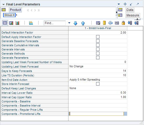
The Final Level view allows you to set the advanced parameters for the final-level forecasts. Figure 8-7 provides an example of a view of this view in a master domain with three partitions/Local Domains, partitioned based on group.
The Final Level Parameters view - Advanced Settings contains the following measures:
Components - Baseline
|
Note: This measure is not displayed for causal levels. |
This measure stores the name of the measure that serves as baseline in the Components forecasting measure. If no measure is specified, the Components forecasting method assesses the value as one (1).
Components - Baseline Interval
|
Note: This measure is not displayed for causal levels. |
This measure stores the name of the measure that serves as baseline interval in the Components forecasting measure. If no measure is specified, the Components forecasting method assesses the value as one (1).
Components - Regular Price Lifts
|
Note: This measure is not displayed for causal levels. |
This measure stores the name of the measure that serves as regular price lifts in the Components forecasting measure. If no measure is specified, the Components forecasting method assesses the value as one (1).
Components - Promotional Lifts
|
Note: This measure is not displayed for causal levels. |
This measure stores the name of the measure that serves as promotional lifts in the Components forecasting measure. If no measure is specified, the Components forecasting method assesses the value as one (1).
Days to Keep Forecasts
This field is used to set the number of days that the system stores forecasts based on the date/time the forecast is generated. The date/time of forecast generation is also referred to as birth date of the forecast. A forecast is deleted from the system if the birth date plus the number of days since the birth date is greater than the value set in the Days to Keep Forecast parameter. This process occurs when either the Forecast Batch Run Workbook wizard is used to generate the forecast or when PreGenerateForecast is executed.
When you start the Forecast Batch Run Workbook, one of the first steps that RDF takes is to remove forecasts older than the value given in the Days to Keep Forecasts parameter. RDF uses the value of that parameter in your local domain. However, because forecasts are registered globally, the Forecast Delete has a global effect. That is, if you set the parameter to some low value, for example, one day, all forecasts in all local domains older than one day are removed. This can adversely impact other users of the system if done without consideration.
When the PreGenerate utility is used, typically for automated batch production of forecasts, RDF uses the value for the Days to Keep Forecasts parameter in the first local domain. Again, if this is set to a value that is not expected by the other users, it can cause unintended disruption.
Refer to the Oracle Retail Demand Forecasting Implementation Guide for more information on PreGenerateForecast.
Default Apply Interaction Factor
When generating the forecast, there are three possible lifts added on top of the baseline to get the final result. They are promotion lift, regular price change lift, and demand transference lift. The Default Apply Interaction Factor measure allows you to specify at a high level if these individually calculated lifts should interact with each other during the forecast generation. This parameter serves as a global setting, but can be overridden at lower levels.
A check in this field (set to True) indicates if you want RDF to combine the promotion, regular price, and demand transference lifts. The impact of the combination can be adjusted in the Default Interaction Factor measure.
Otherwise, by clearing the box (set to False) these effects will be linearly added to the baseline to generate the forecast. By default, the value is set to False. The calculated lifts can be viewed in the Forecast Approval Workbook.
Default Interaction Factor
The Interaction Factor is applied only if the Default Apply Interaction Factor measure is set to True.
This Default Interaction Factor specifies at a high level how the individually calculated promotion lift, regular price change lift and demand transference lift interact with each other during the forecast generation process. This parameter serves as a global setting, but can be overridden at lower levels. The default value is 2.
A value equal to 1 means that each lift will be summed up to calculate the total lift.
A value greater than 1 means the lifts will be compressed when applied in the model, instead of linearly summing up to get the total lift. The larger the value is, the larger the compression effect will be, meaning the smaller the total lift will be.
A value between 0 and 1 means the lifts will be amplified when applied in the model, instead of linearly summing up to get the total lift. The smaller the value is, the larger the amplification effect will be, meaning the larger the total lift will be.
Note that if Apply Interaction Factor is set to True and the Interaction Factor is set to a value other than 1, you should expect to see the combined effects for Demand Transference, Promotion, and Regular Price in the Forecast Approval Workbook.
Default Keep Last Changes
This field is a list from which you select the default change policy for forecast items. Valid values are:
| Field | Description |
|---|---|
| Keep Last Changes (None) | There are no changes that are introduced into the adjusted forecast. The adjusted forecast is equal to the system forecast. |
| Keep Last Changes (Total) | This method allows you to keep previous adjusted forecast value if there is any adjustment existing. For each product/location/week in the forecast horizon, when the last approved system forecast is different from last approved forecast, it means that you have made an adjustment previously. The last approved forecast is used to populated the current adjusted forecast. If the last approved system forecast is the same as last approved forecast, it means that you have not made any adjustment previously and the current adjusted forecast will be populated with current system forecast. |
| Keep Last Changes (Diff) | This method allows you to keep the difference between previous adjusted forecast and system forecast if there is any adjustment existing. For each product/location/week in the forecast horizon, when last approved system forecast is different from last approved forecast, it means that you have made an adjustment previously. The last approved forecast minus the last approved forecast plus the current system forecast is used to populated the current adjusted forecast. If the last approved system forecast is the same as last approved forecast, it means that you have not made any adjustment previously and the current adjusted forecast will be populated with current system forecast. |
| Keep Last Changes (Ratio) | This method allows you to keep the ratio of last adjusted forecast versus the last system forecast if there is any adjustment existing. For each product/location/week in the forecast horizon, when the last approved system forecast is different from last approved forecast, it means that you have made an adjustment previously. The last approved forecast/last approved system forecast multiplied by the current system forecast is used to populated the current adjusted forecast. If the last approved system forecast is the same as last approved forecast, it means that you have not made any adjustment previously and the current adjusted forecast will be populated with current system forecast. |
|
Note: Populating adjusted forecast is the 5th step of the "Batch Flow Process in RDF". Populating adjusted forecast happens before forecast approval. At the time of applying keep last changes, the approved forecast and approved system forecast contains forecast values from last batch. At that moment, RDF checks the value of approved forecast, approved system forecast and current system forecast to populate the adjusted forecast. Once forecast approval is done, approved forecast and approved system forecast is populated with current forecast values. |
Generate Baseline Forecasts
A check should be indicated in this field (set to True) if the baseline forecast is to be generated to be viewed in any task. This parameter should be set if the level is used for Causal forecasting and the baseline is needed for analysis purposes.
Generate Cumulative Interval
A check in this field (set to True) specifies whether you want RDF to generate cumulative intervals (this is similar to cumulative standard deviations) during the forecast generation process. Cumulative Intervals are a running total of Intervals and are typically required when RDF is integrated with the Oracle Retail Merchandising System. If you do not need cumulative intervals, you can eliminate excess processing time and save disk space by clearing the check box. The calculated cumulative intervals can be viewed within the Forecast Approval Workbook.
Generate Intervals
A check in this field (set to True) indicates that intervals (similar to Standard Deviations) should be stored as part of the batch forecast process. Intervals can be displayed in the Forecast Approval Workbook. If you do not need intervals, excess processing time and disk space may be eliminated by clearing the check box. For many forecasting methods, intervals are calculated as standard deviation, but for Simple, Holt, and Winters the calculation is more complex. Intervals are not exported.
Generate Methods
A check in this field (set to True) indicates that when an ES forecast method is used, the chosen forecast method for each fitted time series should be stored. The chosen method can be displayed in the Forecast Approval Workbook.
Generate Parameters
A check in this field (set to True) indicates that the alpha, level, and trend parameters for each fitted time series should be stored. These parameters can be displayed in the Forecast Approval Workbook.
Interval Cap Lower Ratio
The value entered in this field multiplied by the forecast represents the lower bound of the confidence interval for a given period in the forecast horizon.
Interval Cap Upper Ratio
The value entered in this filed multiplied by the forecast represents the upper bound of the confidence interval for a given period in the forecast horizon.
Item End Date Action
This parameter allows the option for items with end dates within the horizon to have zero demand applied to time series before or after the interim forecast is calculated. The two options are:
| Option | Description |
|---|---|
| Apply 0 After Spreading | This is the default value. Spreading ratios are calculated for time series with no consideration made to the end date of an item. It is after the source forecast is spread to the final-level when zero is applied to the System Forecast. |
| Apply 0 to Interim | For items that have an end date within the forecast horizon, zero is applied to the Interim Forecast before the spreading ratios are calculated. This ensures that no units are allocated to the final-level for time series that have ended. |
Store Interim Forecast
|
Note: This measure is not displayed for causal levels. |
A check should be placed in this field (set to True) if the interim forecast is stored. The Interim Forecast is the forecast generated at the Final Level. This forecast is used as the Source Data within Curve to generate the profile (spreading ratios) for spreading the source-level forecast to the final-level. The interim forecast should only be stored if it is necessary for any analysis purposes.
Updating Last Week Forecast
This field is a list from which you can select the method for updating the Approved Forecast for the last specified number of weeks of the forecast horizon. This option is valid only if the Approval Method Override (set in the Forecast Administration Workbook) is set to Manual or Approve by alert, and the alert was rejected. This parameter is used with the Updating Last Week Forecast Number of Weeks parameter.
| Method | Description |
|---|---|
| No Change | When using this method, the last week in the forecast horizon does not have an Approved Forecast value. The number of weeks is determined by the value set in the Updating Last Week Forecast Number of Weeks parameter. |
| Replicate | When using this method the last week in the forecast horizon is forecast using the Approved Forecast for the week prior to this time period. To determine the appropriate forecast time period, the value set in Updating Last Week Forecast Number of Weeks is subtracted from the Forecast Length. For example, if your Forecast Length is set to 52 weeks and Updating Last Week Forecast Number of Weeks is set to 20, week 32's Approved Forecast is copied into the Approved Forecast for the next 20 weeks. |
| Use Forecast | When using this method, the System Forecast for the last weeks in the forecast horizon is approved. |
Updating Last Week Forecast Number of Weeks
The Approved Forecast for the last weeks in the forecast horizon is updated using the method specified from the Updating Last Week Forecast list.
The Final and Source Level view allows you to set the advanced parameters that are common to both the final and source-level forecasts.
|
Note: This view is not available for causal levels. |
The Source Level View - Advanced Settings contains the following measures:
Bayesian Alpha (range (0, infinity))
When using the Bayesian forecasting method, historic data is combined with a known sales plan in creating the forecast. As POS data comes in, a Bayesian forecast is adjusted so that the sales magnitude is a weighted average between the original plan's scale and the scale reflected by known history. This parameter displays the value of alpha (the weighted combination parameter). An alpha value closer to one (or infinity) weights the sales plan more in creating the forecast, whereas alpha closer to zero weights the known history more. The default is one (1).
Bayesian Cap Ratio
The Bayesian Cap ratio is used to cap the resulting Bayesian forecast if it deviates significantly from the sale plan. The Bayesian Cap ratio is used as follows:
Example 8-1
If forecast I > Bayesian Cap ratio * Max value of Past Sales AND
forecast I >  Bayesian Cap ratio * Max value of Past Plan AND
forecast I >  Bayesian Cap ratio * Plan I
then
forecast I  = Plan I
It defaults to a value of 1.5.
Croston's Min Gaps
The Croston's Min Gaps is the default minimum number of transitions from non-zero sales to zero sales. Thus, if Croston's Min Gap is set to five, then the method may fit if you have five or more transitions from non-zero sales to zero sales If there are not enough gaps between sales in a given product's sales history, the Croston's model is not considered a valid candidate model. The system default is five minimum gaps between intermittent sales. The value must be set based on the calendar dimension of the level. For example, if the value is to be 5 weeks, the setting for a final-level at day is 35 (5x7days) and a source-level at week is 5.
DD Duration (weeks)
Used with Profile Based forecast method, the DD Duration is starting from the first week of populated history, the number of weeks of seasonal profiles required after which the system stops using the DD (De-seasonalized Demand) approach and defaults to the normal Profile-Based method. The value must be set based on the calendar dimension of the level. For example, if the value is to be 10 weeks, the setting for a final-level at day is 70 (10x7days) and a source-level at week is 10.
Default Moving Average Window Length
Used with Moving Average forecast method, this is the Default number of data points in history used in the calculation of Moving Average. This parameter can be overwritten at item/location from the Forecast Maintenance Workbook.
Deseasonalized Demand Array
Enter the name of the measure that serves as the deseasonalized data source in the profile-based forecasting method. If left blank, the system uses the forecast data source in combination with a seasonal profile to generate the deseasonalized demand.
Extra Week Interpret Method
This measure indicates how the forecasting value should be calculated if for a week that was flagged extra, or 53rd. This is necessary when an extra week is added within the forecast horizon, because initially no value is calculated for that week.
The options to calculate the value are:
Use average: the value for the extra week is calculated as the average of the values of the weeks immediately prior and after the flagged week.
Use before: the value for the extra week is a replication of the value in the previous week
Use after: the value for the extra week is equal to the value of the following week
Extra Week Indicator Data Source
This measure stores the name of the measure that indicates which week is the 53rd, or extra week. To set this measure, use the Extra Week Indicator found in the Extra Week Administration Workbook.
Fit Error Factor Source
The measure stores the measure name that error factor of sales vs forecast. This measure needs to be at the intersection of the final forecast level, less the calendar dimension, example, item/store.
The Error Factor is necessary for the calculation of the Confidence Intervals.
For the majority of the forecasting methods, the error factor is calculated during forecast generation, but for the following methods the calculation is not possible and needs to be input:
Copy
LoadPlan
Component
Fallback Method
Set this parameter only if the Fallback Method is to vary from the default Fallback Methods used by the selected forecasting algorithm. If the method selected as the Default Forecast Method or Forecast Method Override does not succeed for a time series, this method is used to calculate the forecast and the default Fallback Methods in the forecasting process is skipped entirely. The default Fallback Methods are as follows:
Table 8-1 Fallback Methods
| Fallback Method | Steps |
|---|---|
|
If either the Causal, Bayesian, or Profile-Based are selected as the Default Forecast Method or Forecast Method Override and the method does not fit the data. |
|
|
If the SeasonalES is selected as the Default Forecast Method or Forecast Method Override and neither Multiplicative Seasonal or Additive Seasonal fits the data. |
|
|
If either the Multiplicative Seasonal or Additive Seasonal are selected as the Default Forecast Method or Forecast Method Override and the method does not fit the data. |
|
|
If the TrendES is selected as the Default Forecast Method or Forecast Method Override and the method does not fit the data. |
|
Holt Min Hist (Periods)
Used with the AutoES forecast method, Holt Min Hist is the minimum number of periods of historical data necessary for the system to consider Holt (TrendES) as a potential forecasting method. RDF fits the given data to a variety of AutoES candidate models in an attempt to determine the best method; if not enough periods of data are available for a given item, Holt is not be considered as a valid option.
The system default is 13 periods. The value must be set based on the calendar dimension of the level. For example, if the value is to be 13 weeks, the setting for a final-level at day is 91 (13x7days) and a source-level at week is 13.
Max Alpha (Profile) (range [0.001 to 1])
In the Profile-based model-fitting procedure, alpha, which is a model parameter capturing the level, is determined by optimizing the fit over the de-seasonalized time series. The time series is de-seasonalized based on a seasonal profile. This field displays the maximum value (that is, cap value) of alpha allowed in the model-fitting process. An alpha cap value closer to one (1) allows more reactive models (alpha = 1, repeats the last data point), whereas alpha cap closer to zero (0) only allows less reactive models. The default is one (1).
The value for the optimized alpha parameter will be in the range 0.001 to Max Alpha.
Max Alpha (Simple, Holt) (range [0.001 to 1])
In the Simple or Holt (TrendES) model-fitting procedure, alpha (a model parameter capturing the level) is determined by optimizing the fit over the time series. This field displays the maximum value (cap value) of alpha allowed in the model-fitting process. An alpha cap value closer to one (1) allows more reactive models (alpha = 1, repeats the last data point), whereas alpha cap closer to zero (0) only allows less reactive models. The default is one (1).
The value for the optimized alpha parameter will be in the range 0.001 to Max Alpha.
Max Alpha (Winters) (range [0.001 to 1])
In the Winters (SeasonalES) model-fitting procedure, alpha (a model parameter capturing the level) is determined by optimizing the fit over the time series. This field displays the maximum value (cap value) of alpha allowed in the model-fitting process. An alpha cap value closer to one (1) allows more reactive models (alpha = 1, repeats the last data point), whereas alpha cap closer to zero (0) only allows less reactive models. The default is one (1).
The value for the optimized alpha parameter will be in the range 0.001 to Max Alpha.
Max Gamma (Holt) (range [0,1])
In the Holt (TrendES) model-fitting procedure, gamma (a model parameter capturing the trend) is determined by optimizing the fit over the time series. This field displays the maximum value (cap value) of gamma allowed in the model-fitting process.
The value for the optimized gamma parameter will be in the range 0.001 to Max Gamma.
Max Gamma (Winters) (range [0,1])
In the Winters (SeasonalES) model-fitting procedure, gamma (a model parameter capturing the trend) is determined by optimizing the fit over the time series. This field displays the maximum value (cap value) of gamma allowed in the model-fitting process.
The value for the optimized gamma parameter will be in the range 0.001 to Max Gamma.
Seasonal Smooth Index
This parameter is used in the calculation of seasonal index. The current default value used within forecasting is 0.80. Changes to this parameter impacts the value of seasonal index directly and impact the level indirectly. When seasonal smooth index is set to one (1), seasonal index is closer to the seasonal index of last year sales. When seasonal smooth index is set to zero (0), seasonal index is set to the initial seasonal indexes calculated from history.
This parameter is used for Oracle Winters.
Trend Damping Factor (range [0,1])
This parameter determines how reactive the forecast is to trending data. A value close to zero (0) is a high damping, while a value of one (1) implies no damping. The default is 0.5.
Winters Min Hist (Periods)
Used with the AutoES forecast method, the value in this field is the minimum number of periods of historical data necessary for Winters to be considered as a potential forecast method. If not enough years of data are available for a given time series, Winters is not used. The system default is two years of required history. The value must be set based on the calendar dimension of the level. For example, if the value is to be 104 weeks/2 years, the setting for a final-level at day is 728 (104 weeks x 7 days) and a source-level at week is 104.
Winters Mode
When any forecast method calls multiplicative or additive Winters, the system executes the Oracle Winters forecasting approach.
Winters Mode Impact on AutoES and Causal
The Winters Mode measure determines which Forecasting Approach to use within AutoES and Causal. Also, the errors that are used to calculate the BIC may be different for different Forecasting Approaches and could impact the choice of Forecast Method within AutoES and Causal.
It is recommended that you choose a Forecasting Approach that best suits the nature of your business. The default forecasting approach is Oracle Winters. For additional information on the forecasting approaches, refer to the Forecasting Methods Available in RDF section.
|
Note: If patching this change into a domain, in order to view this measure in the Forecast Administration Workbook, you must add it to the Final and Source Level Parameters View - Basic Settings by selecting it from the Show/Hide dialog within the RPAS Client. |
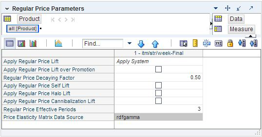
The Regular Price Parameters view allows you to set the parameters that allow you to incorporate the effects of regular price changes within the forecast.
The Regular Price Parameters View- Advanced Settings contains the following measures:
Apply Regular Price Lift
This parameter serves as a global setting, but can be overridden at lower levels.
Select a value from the list for this parameter:
Do Not Apply— no regular price lifts are incorporated in the forecast
Apply System — the effects calculated in RDF are incorporated in the forecast
Apply Override — the lifts calculated in RDF are ignored and the override lifts are incorporated
There are three components to the Regular Price Lift:
Self Lift — determined by the regular price self elasticity
Cannibalization — determined by the regular price cannibalization cross elasticity
Halo — determined by the regular price halo cross elasticity
Apply Regular Price Lift over Promotion
Is only effective if Apply Regular Price Lift is set to Apply System or Apply Override. Place a check in this parameter (set to True) if the application of regular price lifts is enabled for time periods that are promoted. If the parameter is not checked, regular price lifts will not be applied for periods with promotions. This parameter serves as a global setting, but can be overridden at lower levels.
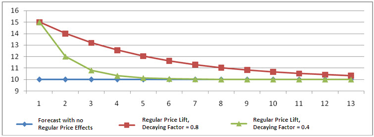
Regular Price Decaying Factor
This parameter determines how the magnitude of the price effects is applied over time.
A regular price change usually triggers a change in demand. However, the effect can be seen only for a few periods following the price change. An adjustable damping mechanism ensures that the regular price effect trends down as time goes by. The decaying factor is a number between zero (0) and one (1).
The closer the decaying factor is to zero (0), the faster the regular price effect decays.
Apply Regular Price Self Lift
Is only effective if Apply Regular Price Lift is set to Apply System or Apply Override. Place a check in this parameter (set to True) if the application of regular price self lifts is enabled for the forecast level. This parameter serves as a global setting, but can be overridden at lower levels.
Apply Regular Price Halo Lift
Is only effective if Apply Regular Price Lift is set to Apply System or Apply Override. Place a check in this parameter (set to True) if the application of regular price Halo lifts is enabled for the forecast level. This parameter serves as a global setting, but can be overridden at lower levels.
Apply Regular Price Cannibalization Lift
Is only effective if Apply Regular Price Lift is set to Apply System or Apply Override. Place a check in this parameter (set to True) if the application of regular price cannibalization lifts is enabled for the forecast level. This parameter serves as a global setting, but can be overridden at lower levels.
Regular Price Effective Periods
Specifies the number of periods for which the regular price effect is applied.
Price Elasticity Matrix Data Source
Specifies the name of the measures that stores the regular price elasticities, such as gammas (rdfgamma). The measure name is implementation specific.
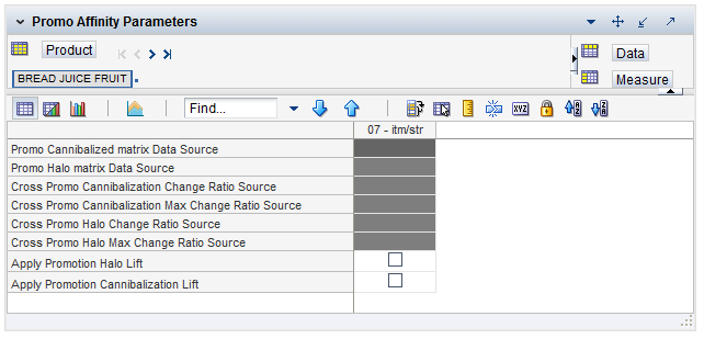
The Promo Affinity Parameters View- Advanced Settings allows you to set parameters to decide if cross promotional elasticities are incorporated in the forecast.
The Promo Affinity Parameters View- Advanced Settings contains the following measures:
Apply Promotion Cannibalization Lift
Select this parameter (set to True) if the application of Cannibalization lifts is enabled for the forecast level. This parameter serves as a global setting, but can be overridden at lower-levels.
Apply Promotion Halo Lift
Select this parameter (set to True) if the application of Halo lifts is enabled for the forecast level. This parameter serves as a global setting, but can be overridden at lower-levels.
Cross Promo Cannibalization Change Ratio Source
This parameter contains the name of the measure that determines the percentage of the promotional lift that is going to cannibalize related items.
|
Note: This measure is specified at an intersection higher than item/store. The content of the measure is visible if you roll up to All Products on the product hierarchy. At a lower intersection the cell appears as a hash mark. |
Cross Promo Cannibalization Max Change Ratio Source
This parameter contains the name of the measure that determines an item's maximum allowed drop in sales due to cannibalization. For instance if the sales of an item for a given period are 20 units, and the maximum allowed percentage is 20%, the drop in sales due to cannibalization for the period can not exceed 4 units.
|
Note: This measure is specified at an intersection higher than item/store. The content of the measure is visible if you roll up to All Products on the product hierarchy. At a lower intersection the cell appears as a hash mark. |
Cross Promo Halo Change Ratio Source
This parameter contains the name of the measure that determines the percentage of the promotional lift that is going to increase demand of complimentary items due to halo effect.
|
Note: This measure is specified at an intersection higher than item/store. The content of the measure is visible if you roll up to All Products on the product hierarchy. At a lower intersection the cell appears as a hash mark. |
Cross Promo Halo Max Change Ratio Source
This parameter contains the name of the measure that determines an item's maximum allowed increase in sales due to halo. For instance if the sales of an item for a given period are 15 units, and the maximum allowed percentage is 20%, the increase in sales due to halo for the period can not exceed 3 units.
|
Note: This measure is specified at an intersection higher than item/store. The content of the measure is visible if you roll up to All Products on the product hierarchy. At a lower intersection the cell appears as a hash mark. |
Promo Cannibalized Matrix Data Source
This parameter contains the name of the measure that is used to spread the cannibalization lift caused by a promoted item to the related items.
|
Note: This measure is specified at an intersection higher than item/store. The content of the measure is visible if you roll up to All Products on the product hierarchy. At a lower intersection the cell appears as a hash mark. |
Promo Halo Matrix Data Source
This parameter contains the name of the measure that is used to estimate the Halo effects between items. The measure name is implementation specific.
|
Note: The content of the measure is visible if you roll up to All Products on the product hierarchy. At a lower intersection the cell is unavailable. |
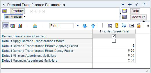
The Demand Transference Parameters View- Advanced Settings allows you to set parameters to decide if and how demand transference is incorporated in the forecast.
The Demand Transference Parameters View- Advanced Settings contains the following measures:
Default Apply Demand Transference Effects
A check in this field (set to True) indicates that RDF will incorporate demand transference in the forecast. Otherwise, by clearing the box (set to False), no demand transference is incorporated in the forecast generation process. The Demand transference function will be enabled if Demand Transference Enabled is specified during implementation, and Default Apply Demand Transference is set to True. This measure serves as a global setting, but can be overridden at lower levels.
RDF loads assortment multipliers from ORME (Oracle Retail Modeling Engine). The demand transference effects are derived from these assortment multipliers, at a prod/loc/clnd intersection. Before RDF incorporates the effects in the forecast, the value of the assortment multipliers can be checked and capped.
If the loaded value is smaller than the Maximum Assortment Multiplier, but greater than the Minimum Assortment Multiplier, the loaded value is applied for the demand transference effect calculation.
Default Demand Transference Effect Decay Factor
This measure is applied if and only if the demand transference function is enabled and applied. This parameter serves as a global setting, but can be overridden at lower levels.
This parameter determines how the magnitude of the demand transference effects is applied over time. An assortment change usually triggers a transference in demand. However, the effect can be seen only for a few periods following the assortment change. In addition, an adjustable damping mechanism ensures that the demand transference effect trends down as time goes by. The decaying factor is a number between zero (0) and one (1).
RDF loads assortment multipliers from ORME (Oracle Retail Modeling Engine). The demand transference effects are derived from these assortment multipliers, at a prod/loc/clnd intersection. Before RDF incorporates the effects in the forecast, the value of the assortment multipliers can be checked and capped.
The closer the decaying factor is to zero (0), the faster the demand transference effect decays.
Default Demand Transference Effects Applying Period
This measure is applied only if the demand transference function is enabled and applied. This parameter serves as a global setting, but can be overridden at lower levels.
This integer measure specifies the number of periods for which the demand transference effect is applied. An assortment change usually triggers a transference in demand. However, the effect is usually seen only for a few periods following the assortment change. The number of periods is specified as an integer in this cell.
Default Maximum Assortment Multipliers
This measure is applied if and only if demand transference function is enabled and applied. This parameter serves as a global setting, but can be overridden at lower levels. It is used to set the maximum threshold of the assortment multipliers.
If the loaded value is greater than the Maximum Assortment Multiplier, the Maximum Assortment Multiplier is applied for the demand transference effect calculation.
If the loaded value is smaller than the Maximum Assortment Multiplier but greater than the Minimum Assortment Multiplier (link), the loaded value is applied for the demand transference effect calculation.
Default Minimum Assortment Multipliers
This measure is applied if and only if demand transference function is enabled and applied. This parameter serves as a global setting, but can be overridden at lower levels. It is used to set the minimum threshold of the assortment multipliers.
If the loaded value is smaller than the Minimum Assortment Multiplier, the Minimum Assortment Multiplier is applied for the demand transference effect calculation.
If the loaded value is greater than the Minimum Assortment Multiplier but smaller than the Maximum Assortment Multiplier (link), the loaded value is applied for the demand transference effect calculation.
Demand Transference Enabled
This read-only measure specifies if demand transference is configured for the final level. The decision to enable demand transference is made in the Configuration Tools.
|
Note: The content of the measure is visible if you roll up to All Products on the product hierarchy. At a lower intersection the cell is unavailable. |
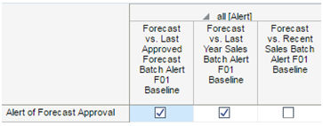
In this view, you can select the batch alerts that can be used for forecast approval. The available alerts are described in detail in the XXX workbook.
However, not all alerts are relevant when used to approve a certain type of forecast. For instance, for the baseline, the following are common choices:
Forecast vs last approved forecast – also available as a real time alert
Forecast vs sales last year – also available as a real time alert
Forecast vs recent sales
Upon making the selection of the alerts to be used for approving the baseline forecast, click Calculate to update the approval list to reflect your choices:
For the causal level, relevant approval alerts are:
Causal peaks – also available as a real time alert
Forecast vs last approved forecast – also available as a real time alert
Upon making the selection of the alerts to be used for approving the causal forecast, click Calculate to update the approval list to reflect your choices: