Pivot Your Dataset Query Results
If you haven't already, complete Step Four: Create a Workbook Based on Your Dataset.
The following steps show you how to pivot your dataset query results to create a pivot table.
To pivot your source data:
-
On the Pivot tab, drag fields from the Fields list to the Rows, Columns, or Measures tabs in the Layout panel. Or, drag them straight into the Pivot Table Viewer.
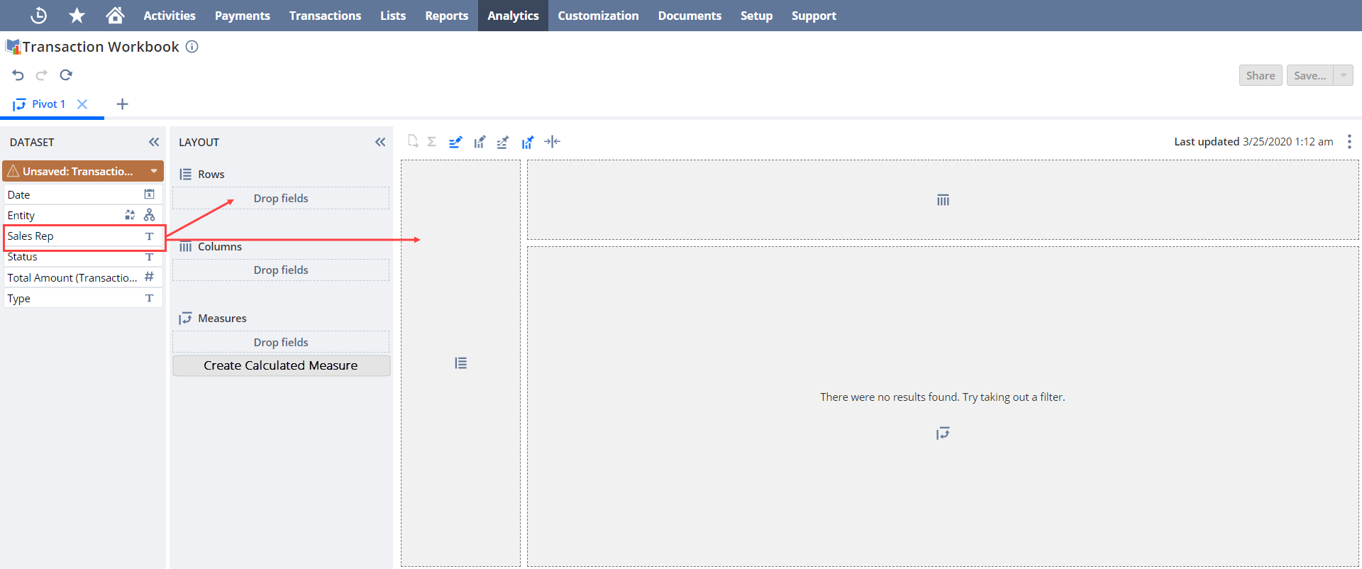
For this tutorial, add the item and status fields to Rows, and add the amount (net) and quantity fields in Measures.
Note:If you add hierarchical fields, you'll be prompted to pick a display type for them. Based on where you add the field and the display type, you can add subtotals at each level. For more information, see Hierarchical Fields.
-
(Optional) To created a calculated measure, click Create Calculated Measure in the Layout Panel. You can also click the Field Menu icon
 next to a measure in the Pivot Table Viewer and select Create Calculated Measure. Calculated measures are displayed with a calculator icon
  . For more information, see Calculated Measures.
 -
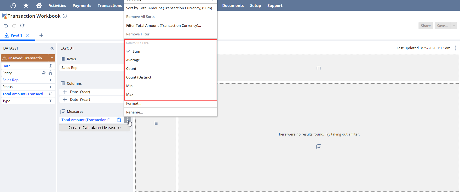
Select the summary type and format options for any date or numerical fields you add to the pivot table.
-
Click the Field Menu icon
next to the field you want to format in the Layout panel. -
Select a summary type from the popup window.
-
(Optional) Select Currency... to view the currency consolidation or conversion options for fields with values in multiple currencies.
For more information, see Currency in Datasets and Workbooks.
Important:If your fields have values in multiple currencies, you'll need to convert them to a single currency before doing arithmetic or any numeric manipulation.
-
(Optional) Click Format... to customize the numeric values for a field.
For more information about numeric formatting options, see Customizing Numeric Values.
For the purposes of this tutorial, select the following summary types. No numeric formatting is required:
-
Amount (Net) (Sum)
-
Quantity (Sum)
-
-
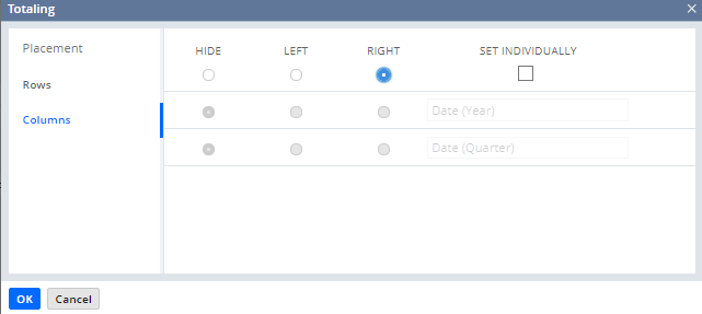
Add totals and grand totals to the pivot table.
-
Click the Totaling icon
 .
. -
In the Totaling window, select where you want the totals or grand totals for each field to appear. If there are multiple fields that can be totaled in the rows or columns, check the Set Individually box to choose where the totals for each field appear on the pivot table.
-
Click OK.
For the purposes of this tutorial, no totals are required.
-
-
Click the Refresh icon
 to generate the pivot table.
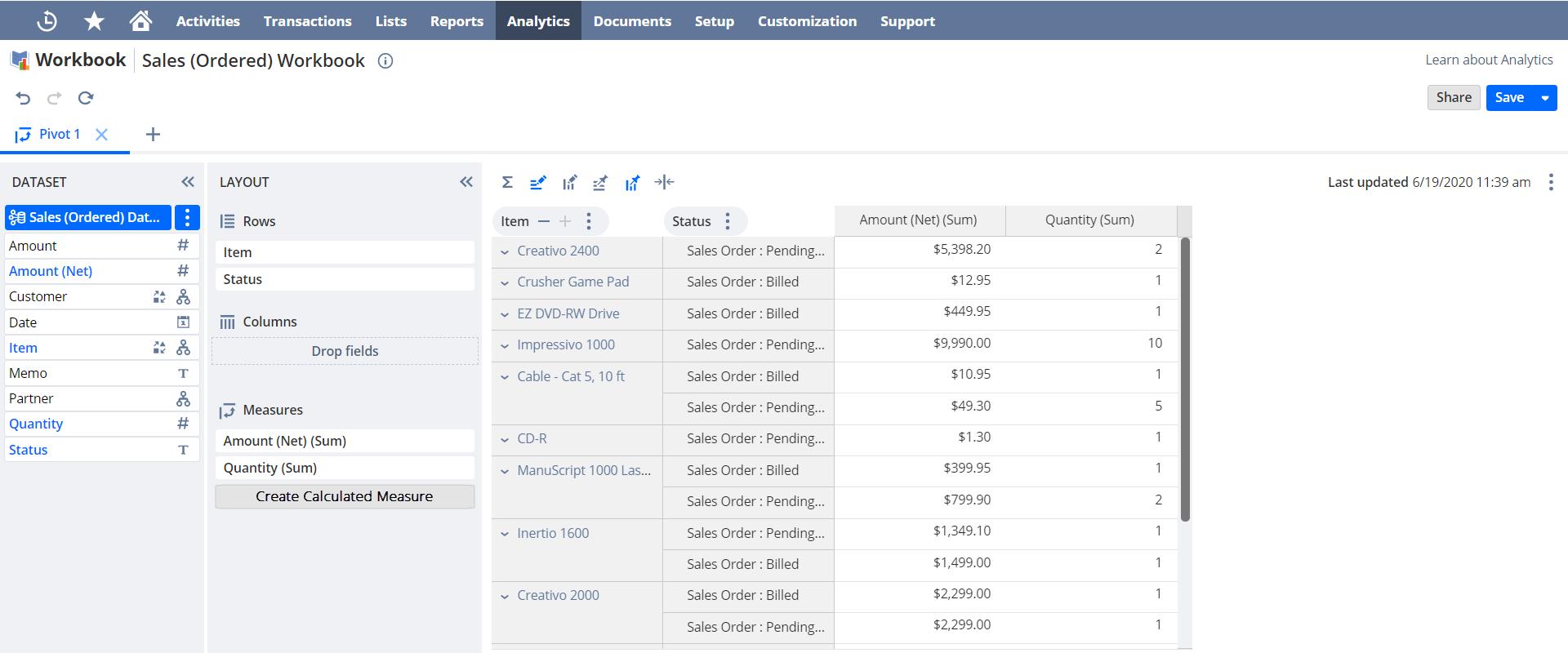
-
(Optional) Filter the data displayed in the pivot table.
Note:Filter conditions created on the Pivot tab only affect the data you see in the pivot table. They don't change the underlying dataset or other workbook visualizations.
-
Click the Field Menu icon
next to the field you want to filter. Depending on whether it's set as a column, row, or measure, or if you click the Field menu icon from the Fields List or the Layout Panel, the following options are available:-
Top 10: display only the top 10 rows or columns based on the measures defined for the table.
-
Bottom 10: display only the bottom 10 rows or columns based on the measures defined for the table.
-
Filter [Field Name] by...: enables you to define a custom measure-based filter for the selected row or column.
-
Filter [Field Name]: enables you to define a custom value-based filter based on specific values within the table results.
-
Add as Filter...: enables you to define a custom value-based filter based on specific values within the table results.
-
-
The results in the table are updated automatically.
For more information, see Workbook Visualization Filters.
For the purposes of this tutorial, no pivot table filters are required.
-
-
(Optional) Apply conditional formatting to the pivot table measures to highlight your results.
Important:If your measure field has values in multiple currencies, you need to convert or consolidate them before applying conditional formatting. For more information, see Currency in Datasets and Workbooks.
-
Click the Field Menu icon next to the measure field you want to highlight in the Layout Panel and point to Conditional Formatting.
-
Click Manage Conditional Formatting, then select the operators, values, and colors or icons for the rule. You can click the
 add icon to create multiple rules and apply different colors or icons to the same measure or column. For more information, see Conditional Formatting.Note:
To apply conditional formatting to percentage values, use decimal format when defining the values for the rule. For example, rather than greater or equal to 20%, the rule should be defined as greater or equal to 0.2.
-
Check Apply to subtotals and grand totals if you want to apply your rules to the measure subtotals and grand totals.
-
Click Apply.
-
Repeat steps A-D for each measure you want to highlight.
For the purposes of this tutorial, no conditional formatting is required.
-
-
(Optional) Click the Export icon to save a CSV file of your pivot table.
Continue to Step Six: Connect a Second Dataset to Your Workbook.